
Phish by the Numbers
May 21, 2017
“My geekiness is getting in the way of my nerdiness” - Patton Oswalt
Phish is a quartet and stalwarts of the modern jam band scene they helped create in the late 80’s. Like their Deadhead contemporaries, Phish fans (phans) have an almost unhealthy obsession with the music, speaking in reverential tones of near mythical versions of songs, like 2015’s Tweezer -> Prince Caspian, while endlessly debating the details (for the record, no, I do not think they went back into Tweezer). This devotion to the music, an unabiding urge to get a taste of IT, has numerous implications - on bank accounts, relationships (Confessions of a Phish Wife), livers, and, in this case, data.
Coinciding with the emergence of the internet, phans have been compiling, debating, and analyzing Phish data online for literally decades. Whether it’s in the pursuit of tracking your “stats” (shows attended, songs heard, etc.) or quantifying “bust outs” (songs not heard in X many shows), data is no stranger to a Phish discussion. So, from the moment I learned that there are numerous online sources of data about this band I love, the data monkey in my brain has been burning the banana at both ends thinking of ways to, like everything else in my life, over analyze Phish.
Soundcheck
The data for this analysis comes from the following sources who are kind enough to make their data available through application programming interfaces (APIs):
- Phish.net - A project of the non-profit Mockingbird Foundation, an entirely volunteer run foundation started by Phish fans in 1996. If you enjoy this post, please consider making a donation!
- Phish.in - A live Phish audio streaming site and my de facto homepage these days
- Spotify
I access, analyze, and visualize all the data using R, an open source programming language original designed for statistical analyses but that can now make burritos, babysit your kid, and even moderate civil discussions between Trump supporters and Berkeley students. At least it seems that way.
I’ve included certain interesting code blocks below but, for anyone interested in the full code, checkout my GitHub page.
Set 1: The Band
Where does Phish play?
Phish gained popularity the old fashioned way, by making the faces of New England college students melt harder than Nectar’s gravy fries while touring relentlessly in the late ’80s and early ’90s. By the mid ’90s, the Phish from Vermont had built a loyal fan base that, I would argue, remains one of music’s strongest to this day. Along the way, Phish played over hundreds of venues in almost every state. So, which states have Phish shown the most love over the years?
To answer this question, I used data on the number of shows per venue available here at phish.net. I couldn’t find an access point for this data through the .net API, so instead I chose to use the R package rvest to scrape the data from the website itself.
# Scrape table of show counts by venue from phish.net
url <- "https://phish.net/venues"
venues <- url %>%
  read_html() %>%
  html_nodes(xpath='/html/body/div[1]/div[2]/table') %>%
  html_table()
venues <- venues[[1]]
The xpath='/html/body/div[1]/div[2]/table' argument refers to the table element on the page that I’m interested in. You can find this info by left-clicking and using the handy Inspect feature in Chrome. For more about using rvest to scrape data from the web, see this helpful post by Cory Nissen.
# Get data for state map
states <- map_data(map = 'state')
state_info <- data_frame(region = state.name,
                         state      = state.abb)

# Summarize shows by state and join with map data
state_shows <- venues %>%
  tbl_df() %>%
  group_by(State) %>%
  summarize(shows  = sum(`Times Played`, na.rm = T),
            venues = length(`Venue Name`)) %>%
  rename(state = State) %>%
  left_join(state_info) %>%
  mutate(region  = tolower(region),
         percent = 100 * shows / sum(shows, na.rm = T)) %>%
  arrange(desc(shows))
Next, I summarized the venue data to see how many shows and different venues Phish has played in each state (Figure 1).
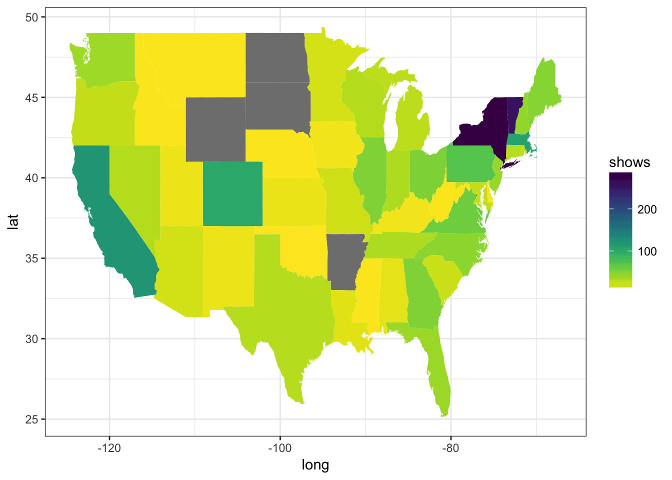
Figure 1: Map of Phish performances by State
New York (283 shows; 97 venues) and Vermont (259 shows; 68 venues) are the clear winners and collectively home to 542% of all Phish shows. California (119 shows; 55 venues), Colorado (114 shows; 83 venues), and Massachusetts (105 shows; 43 venues) are also no stranger to a Phish show. Wyoming, the Dakotas, and Arkansas…not so much.
What does Phish play?
One thing I always get a kick out of is watching the mental gymnastics people go through trying to comprehend how someone could see the same band multiple (13?) nights in a row, or 20, 40, 50, 100, 200+ times in their life. Some people get it, some people don’t, and when people don’t get it it’s almost as if you told them you pour milk in the bowl before the cereal. Utter madness. However, when the band your seeing has a catalog larger than Donald Trump’s supply of artificial tanner, every show is different. That being said, which songs do Phish play the most? Again, I turned to phish.net to find the number of performances of each song.
# Get data from Phish.net
songs <- read_html('http://phish.net/song/')

# Get show table
songs_df <- songs %>%
  html_nodes('#song-list') %>%
  html_table(fill = T)
songs_df <- songs_df[[1]]

# Prep data for wordcloud
songs_df <- songs_df %>%
  mutate(Times = as.numeric(Times),
         word  = as.factor(`Song Name`)) %>%
  rename(freq = Times) %>%
  select(word, freq) %>%
  filter(is.na(freq)==F & freq > 0)
I’m a fan of using word clouds. I’m also a fan of the movie The Life Aquatic With Steve Zissou. So here’s a word cloud of the most played Phish songs using Steve Zissou’s favorite colors, courtesy of the wonderfully random wesanderson R package.
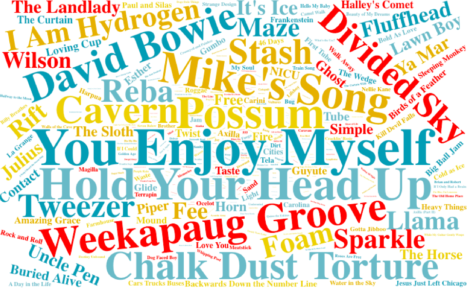
Figure 2: Word cloud of Phish songs sized by number of performances
Not surprisingly, You Enjoy Myself, Phish’s pièce de résistance, is also their most performed song. Staples like Possum, Mike’s Song, Weekapaug Groove, Reba, Divided Sky, and Tweezer are also prominently displayed. Meanwhile, good luck finding Destiny Unbound in that thing. I guess even in nerd graphics she’s a rare beauty.
There’s a lifetime of music represented in the word cloud above, but simply playing the song is not what continues to attract middle-aged accountants, millennial unpaid interns, and your friendly neighborhood purveyor of heady crystals. It’s the jams. It’s when our favorite guitarist does his best impression of a constipated dentist patient while Mike hits you with the brown note that has kept us coming back and (mostly) speaking their praises for decades.
Set 2: The Jams
Not surprisingly, lists of noteworthy jams are carefully curated by the good folks at Phish.net. These “jamcharts”, together with performance-specific data from phish.in and Spotify, provide a cool opportunity to explore several questions about what makes a good Phish jam.
How long does Phish jam?
Whether it’s an extended psychedelic jam, a hard-hitting micro jam, or a unique rendition (4/5/1998 Cavern anyone?), IT can happen at any time. That being said, Phish has deservedly earned a reputation for “playing the same song forever.” - annonymous Chad. I think it’s a fair assumption that most phans crave that moment where Kuroda drops the lights and [insert song here] melts into uncharted “Type 2” territory. However, whether what emerges from the primal soup tickles your fancy more than when said song stays in it’s lane and smothers itself with extra mustard is, like, just your opinion man. With that said, let’s look at how the length of a song influences it’s chances of being admitted to the hallowed halls of the Phish.net jamcharts.
First, I extracted the jamcharts from Phish.net for a set of jam classics, including Tweezer, Bathtub Gin, David Bowie, and Down with Disease.
# Get table of all jamcharts
jc_all <- GET(paste0(end_point,'jamcharts/all?apikey=',api_key)) %>% content
jc_all <- jc_all$response[2]$data

# Convert response to data frame
jc_all <- map_df(seq_len(length(jc_all)), function(x) {
  list(song = jc_all[[x]]$song,
       songid = jc_all[[x]]$songid,
       jams   = jc_all[[x]]$items)})

# Get info for top songs
top_jam_ids <- filter(jc_all, song %in% top_jams)

# Pull jamcharts for top_jam_ids
top_jams_charts <- lapply(top_jam_ids$songid, FUN = jam_chart) %>%
  bind_rows() %>%
  left_join(top_jam_ids)
Next, I joined this data set of ear candy with data from the phish.in API on song length and added labels for jamchart performances as well as for the coveted “Highly Recommended” jams.
# join with Phish.in data on performances
jams <- top_songs %>%
  select(-slug) %>%
  left_join(top_jams_charts) %>%
  mutate(recommended = ifelse(is.na(highly_rec)==F, 'Yes', 'Sure')) %>%
  distinct()

# add label for highly recommended jams
jams$recommended[jams$recommended == 'Yes' & jams$highly_rec == 1] <- 'Highly'
Now let’s look at what our complied data set shows us about the distribution of performances.
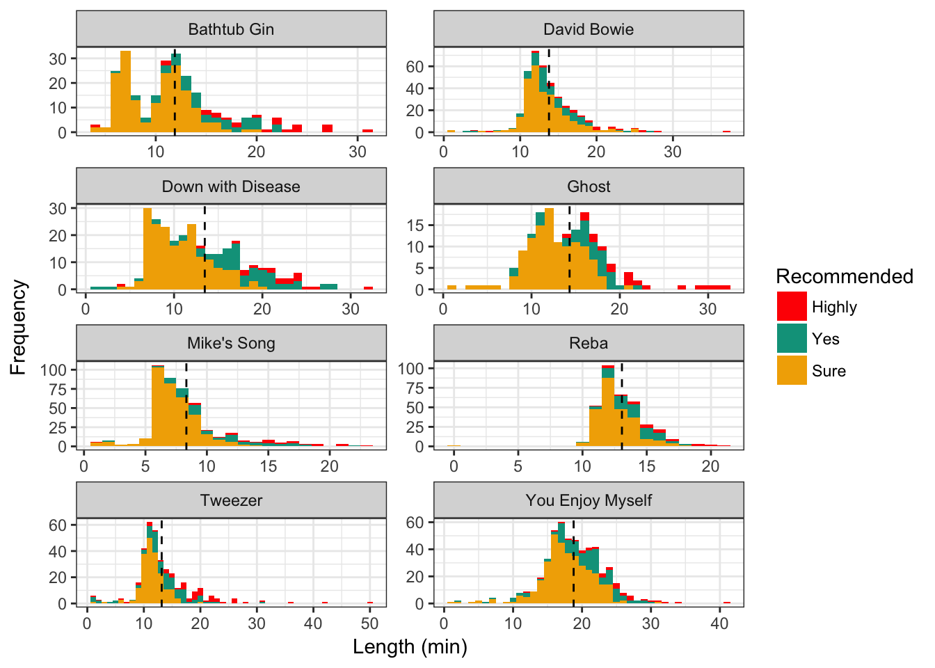
Figure 3: Distributions of performance length and recommendation level
Distinguishing type-1 and type-2 jams is more clear for certain songs than others. The clearest example is the dual peaks to the distribution for Ghost, where a version safely enters type-2 territory after 16 minutes. For other songs, like Bowie and Tweezer, the line between type-1 and type-2 is less clear, and for beloved classics like Reba and You Enjoy Myself you can usually count on surrendering to the flow for around 13 and 18 minutes, respectively (Table 1). Regardless, rest assured that, as each minute passed, you were increasingly likely to be witnessing something special. Also, don’t freak out if that Tweezer you were so stoked to catch bails out after only a few minutes, you may be in store for a highly recommended segue-fest. Lastly, if you witness the boys break the 30 minute mark, congratulations; don’t let your jaw break when it hit’s the floor.
| Song | Performances | Average length | Standard deviation |
|---|---|---|---|
| Bathtub Gin | 275 | 11.89 | 4.81 |
| David Bowie | 412 | 13.77 | 3.71 |
| Down with Disease | 298 | 13.48 | 5.70 |
| Ghost | 183 | 14.31 | 4.61 |
| Mike’s Song | 472 | 8.33 | 3.31 |
| Reba | 377 | 13.07 | 1.97 |
| Tweezer | 381 | 13.16 | 5.25 |
| You Enjoy Myself | 541 | 18.78 | 4.51 |
What Figure 3 and Table 1 don’t show is how performances of these songs changed over time. This is an easy extension, and Figure 4 plots the average performance length of a song by year, with the number of performances indicated by dot size and the dotted line representing the overall average length of each song. The background colors indicate the different Phish “eras”.
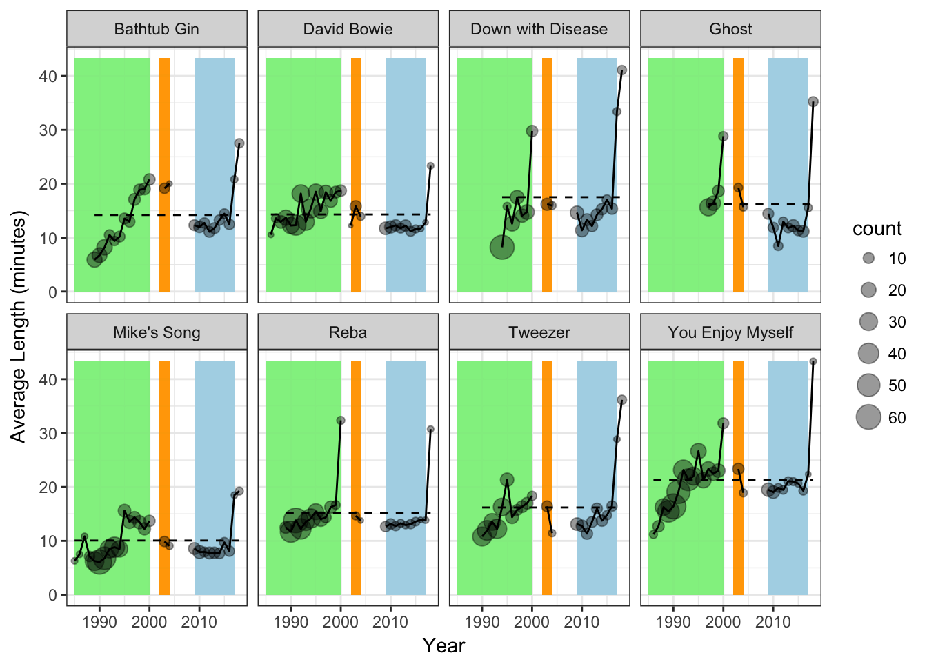
Figure 4: Average performance length by year
It’d be a lie to say the Mike’s Songs and David Bowie’s of today are as exploratory as they were in the ’90s. It’s not all bad news, however, as Down with Disease and Tweezer continue to regularly mix it up, while it would appear the band has really honed their groove in Reba, You Enjoy Myself, and Bathtub Gin over the years.
IT According to Spotify
For my final bit of Phish data nerdery (for now…) I decided to examine what Spotify can tell us about what makes a good Phish jam? (if you haven’t already checked out Charlie Thompson’s excellent analysis, Finding Radiohead’s most depressing song, I highly recommend you do so). All Spotify tracks receive scores for numerous metrics that, I assume, Spotify uses in their noble quest to help you discover new music (seriously, the Discover Weekly, Your Daily Mix, and Release Radar playlists are fantastic). These metrics include things such as energy, danceability, instrumentalness, liveness, valence (how “happy” a song sounds), key, and tempo.
As a first step, I extracted and plotted the key metrics for every live Phish song available from the Spotify API (Figure 5).
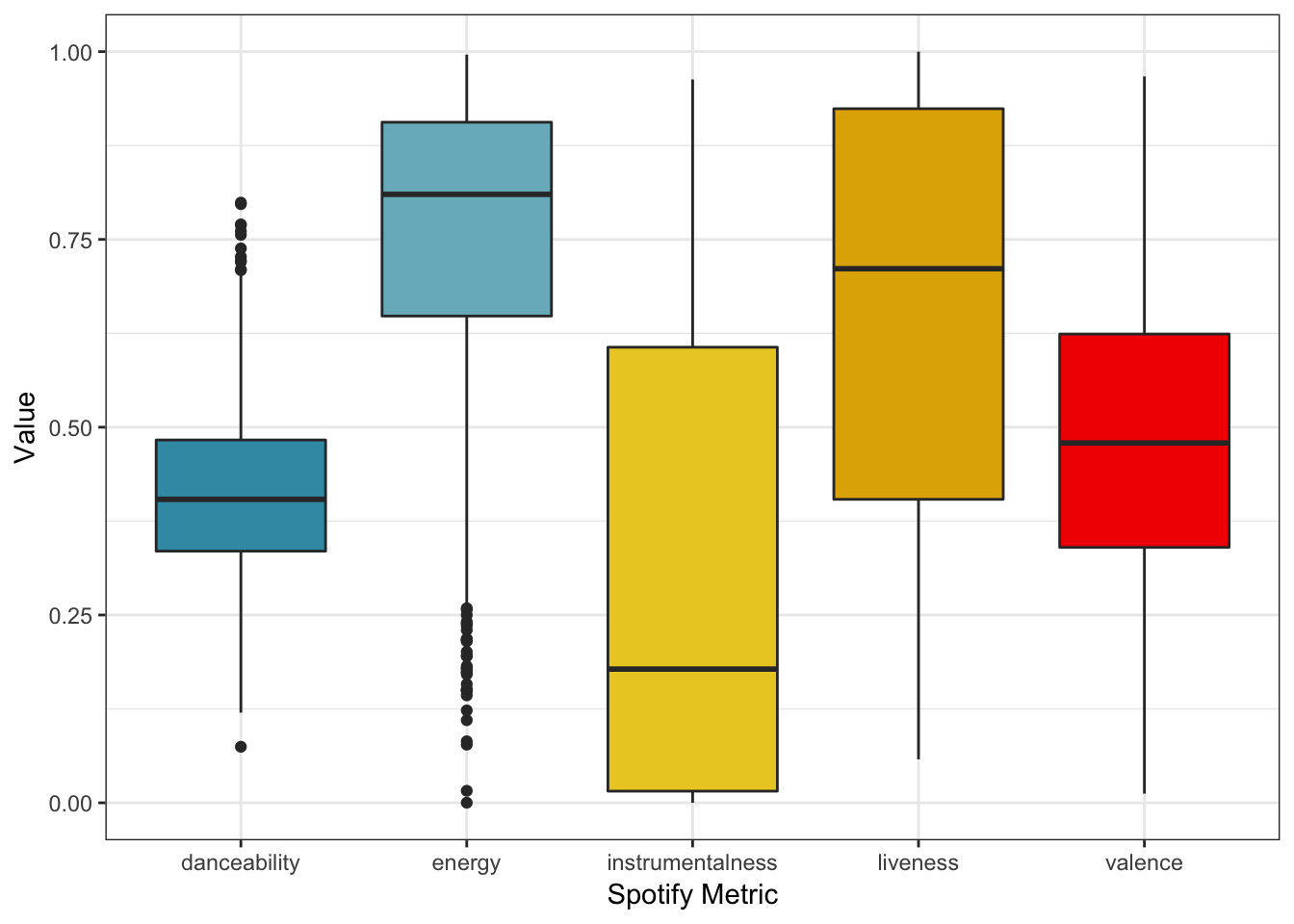
Figure 5: Spotify metrics for all Phish live performances available on Spotify
Now, I don’t work for Spotify and don’t know how they score these things, but when I see instrumentalness as the lowest scoring metric I immediately think alternative-facts. According to the documentation, which you can read here if you’re curious, instrumentalness scores are more of a measure of the presence of vocals and not instrumental prowess. Why they didn’t go with a name like, oh I don’t know, vocals is a bit of a mystery. You may also be wondering why I chose to include liveness considering all the tracks are, well, live. The liveness metric measures the presence of an audience in a track, which I decided could be a good way to gauge audience reaction to a jam. This likely has problems for set-opening and closing tracks, but oh well.
Anyway, instrumentalness rant aside, the rest of the scores generally make sense to me - high energy, below average danceability (unless you’re dancing style is classic white dude like mine), high audience engagement, and songs that take you on a trip across the entire range of emotions (valence). These patterns also seem to be generally consistent across different songs (Figure 6).
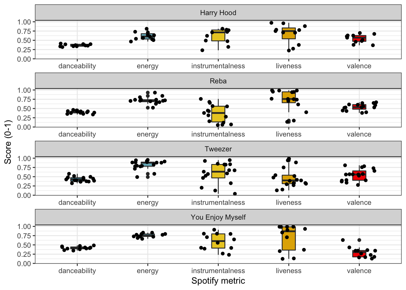
Figure 6: Spotify metrics for all performances available of select Phish songs
At this point, we can combine Spotify’s track metrics with our previous data set of jamchart versions of songs to create a data set with which to ask the question what makes a good Phish jam?
Disclaimer - I’ll preface this by saying the following analysis is more meaningless than truth and integrity are to Paul Ryan. This data monkey Phish phan knows that no amount of number crunching can capture what makes a particular jam special.
The first step is to flag all Spotify songs that are deemed Highly Recommended, which is made easy thanks to the awesome Spotify playlist Phish.net “Highly Recommended”. If you’re a Phish phan and a Spotify user, good luck listening to anything else for the next three months. Again using the Spotify API, I extracted the track list of all “Highly Recommended” songs. I then added a binary variable to the complete data set of Spotify metrics labeling these versions with a 1 and all others with a 0.
Next, I constructed a series of binary logistic regression models, which can be used in situations where the observed outcome can have only two possible outcomes, in this case “Highly Recommended” (1) or not (0).
The results of all three models are included below in Table 2, and they make me very happy.
| Dependent variable: | |||
| highly_rec | |||
| (1) | (2) | (3) | |
| instrumentalness | 2.139*** | 2.119*** | 2.144*** |
| (0.284) | (0.283) | (0.282) | |
| energy | -0.137 | -0.103 | -0.096 |
| (0.581) | (0.580) | (0.579) | |
| valence | 0.655 | 0.698 | 0.722 |
| (0.541) | (0.538) | (0.536) | |
| minutes | 0.139*** | 0.137*** | 0.135*** |
| (0.017) | (0.017) | (0.016) | |
| liveness | -1.807*** | -1.806*** | -1.806*** |
| (0.332) | (0.331) | (0.331) | |
| danceability | -0.260 | -0.348 | -0.354 |
| (0.975) | (0.968) | (0.966) | |
| key | 0.035 | 0.035 | |
| (0.027) | (0.027) | ||
| tempo | 0.003 | ||
| (0.004) | |||
| Constant | -3.429*** | -3.034*** | -2.859*** |
| (0.774) | (0.632) | (0.616) | |
| Observations | 1,251 | 1,251 | 1,251 |
| Log Likelihood | -428.667 | -429.073 | -429.917 |
| Akaike Inf. Crit. | 875.333 | 874.146 | 873.834 |
| Note: | p<0.1; p<0.05; p<0.01 | ||
So, what makes a good Phish jam? Well, according to Spotify, it’s when the Phish from Vermont take a song for an extended and highly instrumental journey. The results also suggest that positive “bliss” jams put a smile on your face for a reason. This is not to say that the dark and nasty grooves don’t get any love, just ask the Dick’s No Men In No Man’s Land. The energy and danceability of a song don’t preclude it from becoming “Highly Recommended”, which should make the lovers of spacey jams happy.
Well, there you have it, my data nerdery is finished getting in the way of my Phish geekery. If you’re a data person and have questions about my methods or code, let me know. If you’re a Phish phan, I hope you didn’t find this to be too sacrilegious. Either way, let me know what you think in the comments.
I’ll end by saying that I strongly believe you can’t capture IT in a statistic. Besides, my license plate is currently duck-taped to the bumper of my station wagon, so you probably shouldn’t listen to me anyway.
Encore
encore <- as.character(0)