Common errors and debugging R code
December 1, 2018
“PC load letter! What the fuck does that mean?” - Michael Bolton, Office Space
If you’ve ever written code, you’ve also probably spent (easily) twice as much time trying to figure out why it doesn’t work. Maybe you forgot a bracket? Maybe you used the wrong file path? Maybe your code runs just fine, except your model now estimates the global population is 90 billion people and you’re seeing some pesky warning message about vectors of different lengths. Whatever the reason, you will find yourself searching for the gremlin in your code and hoping it doesn’t take you three full work hours (days?) to solve the problem. This post is designed to provide a broad overview of the concepts, tools, tips, and tricks you can use to track down problems in your R code.
General Concepts
Before diving into common errors and available debugging tools for R, let’s review a few general programming concepts that are often the culprits behind many errors.
Working Directory & File Paths
When working in R, we often need to read in a data set and save subsequent results and figures by writing them to the hard drive. Both of these operations require specifying a file path, which refers to a file’s unique location in a file system and can be thought of as the file’s address on your computer. There are two options for specifying a file’s path - the absolute and relative paths - which differ in whether or not they depend on the current working directory. Returning to our address analogy, the working directory refers to the folder (directory) that R considers to be the home address for whatever analysis you’re working on.
R will look for (and save) files to the working directory folder unless told otherwise. Keeping all your files in a single directory can be messy, however, and so we can tell R to read/write data to/from different folders using absolute or relative paths:
- Absolute or “full” paths point to the same location, regardless of the current working directory
- e.g., the
.Rmdfile for this tutorial is located at/Users/Tyler/Desktop/GitHub/tylerclavelle/content/blog/2018-12-01_deBug.Rmdon my computer
- e.g., the
- Relative paths point to the file’s location relative to the current working directory
- e.g., because my working directory is
/Users/Tyler/Desktop/GitHub/tylerclavelle, the relative path for the same.Rmdfile iscontent/blog/2018-12-01_deBug.Rmd - *Note: RMarkdown files are a special exemption. When knitting
.Rmdfiles, R will use the location of the.Rmdfile as the working directory
- e.g., because my working directory is
It is generally a good idea to use relative paths for the purposes of making your work reproducible and easy to collaborate on. Consider two users (or even one user with two computers) attempting to collaborate on a GitHub repository they have each cloned to their computers. Absolute paths will not work properly since they will be different for each computer while relative paths will remain valid. This assumes that all users have specified the same working directory, such as deBug/ in the above example.
You can determine your current working directory with getwd() and can tell R to use a different working directory with setwd('path/to/new/working/directory'). To set a default working directory for your R scripts go to RStudio -> Preferences -> General:
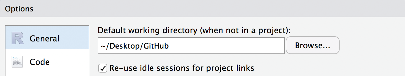
You may be tempted to start each R script by specifying the desired working directory with setwd(). Don’t! This approach can have the same issues with reproducibility/collaboration as absolute paths and, besides, there’s a better way!
RStudio Projects
RStudio Projects are a built-in way to organize all the files associated with a project. There are a lot of advantages to using R Projects that are beyond the scope of this tutorial, so check out the above link to learn more about badassing your RStudio workflow with projects.
Environments
Environments organize a set of name-value bindings. A useful analogy is to think of an environment as a contact list for R objects - the environment contains a list of R objects (the “people”) and their associated values (their “phone numbers”). Understanding environments is critical for debugging code because environments determine what objects (variables, data frames, functions, etc.) are visible to a particular line of code. While a detailed explanation of R environments is beyond the scope of this tutorial, Hadley Wickham (who else?) has this great tutorial available for anyone interested.
For debugging most R errors, the important environments to understand are the global environment (globalenv()) - the interactive workspace in which you normally work - and the current environment (environment()) - the environment containing whatever code is currently being executed. Understanding the difference between these two becomes particularly necessary when using functions. Every time a function is called, R creates an execution enviornment in which to host execution of that function’s code. This environment is a temporary child of the global (or parent) environment; it can access objects (bindings) in its parent environment(s) but bindings created within the execution environment will not become visible to the parent environment(s) unless explicitly assigned with the deep assignment arrow, <<-. The regular assignment arrow, <-, always creates a local variable in the current environment while <<- either modifies an existing variable in the parent environment or creates one in the global environment. The deep assignment arrow will never create a variable in the current environment.
Consider the following example, in which a the function foo() is used to modify both a local and global variable:
# Create global variable
a <- 1

# foo function
foo <- function(x) {
  # create local variable b from global variable a and function argument x
  a <- a + x
  print(a)
}

# Run foo
foo(4)
## [1] 5Running foo(x) prints a value of 5. But if check the value of a outside of the function we see that it is unchanged:
print(a)## [1] 1Syntax vs Semantic Errors
There are two main types of errors in R code:
- Syntax errors result from invalid code statements that R doesn’t understand. Syntax errors will always result in error messages
- Semantic errors result from valid code that successfully executes but produces unintended outcomes
Not surprisingly, syntax errors can be considerably easier to debug than semantic errors since they provide a (sometimes) useful error message and do not suggest an underlying flaw in methodology/logic.
Common Errors & Warnings
One thing that R is notorious for is its often cryptic and difficult to decipher error messages. In what can only be described as an act of masochism, Noam Ross investigated the most common errors in R using data from nearly 20,000 Stack Overflow posts. The results showed that a considerable fraction of problems people have can be attributed to the handful of error types outlined below:
object not found...The object (variable, data frame, list, function, etc.) being called in the code has not actually been defined:
# Try printing foo
print(foo2)
## Error in print(foo2): object 'foo2' not foundCheck spelling and, in the case of objects read from data files, that the file path is correct.
could not find function...The function is spelled wrong or the package it belongs to has not been loaded:
# Create foo (will fail)
foo <- data_frame(x = c(1:5), y = letters[1:5])
## Error in data_frame(x = c(1:5), y = letters[1:5]): could not find function "data_frame"# load tidyverse
library(tidyverse)
# Create foo after loading package (will work)
foo <- data_frame(x = c(1:5), y = letters[1:5])Error in if...The logical statement in yourif()statement is not yielding a logical value (TRUE/FALSE)
if(foo[6,1] > 4) { print('woohoo!')}## Error in if (foo[6, 1] > 4) {: missing value where TRUE/FALSE neededsubscript out of boundsCode refers to an index that does not exist:
# Matrix
a <- 3
foo <- matrix(NA, nrow = 2, ncol = 2)
foo[a,1] <- 'wtf'
## Error in `[<-`(`*tmp*`, a, 1, value = "wtf"): subscript out of boundsNote: This error applies to matrices and lists but NOT data frames or vectors.
# Make foo2 a dataframe instead of a matrix
foo <- data.frame(matrix(NA, nrow = 2, ncol = 2))
# Printing does not give an error, just an NA
foo[a,1]
## [1] NAThis can result in unintended outcomes that go unnoticed, such as accidentally creating the erroneous index in your data frame:
# Assignment will actually CREATE that index in the data frame or vector
foo[a,1] <- 'wtf'
foo
## X1 X2
## 1 <NA> NA
## 2 <NA> NA
## 3 wtf NA...cannot open the connectionR can’t read/write the file, usually due to an incorrect path:
write_csv(foo, path = 'the/long/road/to/nowhere.csv')## Warning in open.connection(path, "wb"): cannot open file 'the/long/road/to/
## nowhere.csv': No such file or directory## Error in open.connection(path, "wb"): cannot open the connectionnon-numeric argument to binary operatorTrying to do math with a non-numeric variable, such as when a data frame column is accidentally a character column:
a <- '7'
6 + a
## Error in 6 + a: non-numeric argument to binary operatorreplacement has...Attempting to assign a vector of values to a subset of an existing object where the lengths are different:
foo <- data_frame(n = c(1:5), d = letters[1:5])
foo$test <- c(1:10)
## Error in `$<-.data.frame`(`*tmp*`, test, value = 1:10): replacement has 10 rows, data has 5# Replacement is longer
a <- c(30:50)
foo <- c(1:30)
foo[1:10] <- a## Warning in foo[1:10] <- a: number of items to replace is not a multiple of
## replacement lengthDebugging Tips & Tools
Time for the (not so) fun stuff - debugging tips and tools. In a nutshell, debugging includes the following steps:
- Locate the point in the code where the error occurs (syntactic errors) or where you suspect it occurs (semantic errors)
- Stop the code at that point
- Examine the code within the context of the current environment
R and RStudio provide a handful of useful built-in tools designed to help you locate an error and investigate the environment state at the time of the error in order to figure out what went wrong.
print is your best friend
It’s hard to overstate the value of the print function to the debugging process. Using print can help you both locate and diagnose a problem in your code.
Consider the following example:
for (a in 1:length(v1)){
  b <- 10 / v1[[a]]
}
## Error in 10/v1[[a]]: non-numeric argument to binary operatorThere’s an error in our for loop, but we’re not sure where. The simple b <- 10 / a is valid code assuming a is numeric, so we suspect there’s a problem somewhere in v1. If v1 is small, a reasonable first step is to just use print(v1) to visually inspect v1 for problems.
print(v1)## [[1]]
## [1] 1
##
## [[2]]
## [1] 2
##
## [[3]]
## [1] "5"
##
## [[4]]
## [1] 6Right away we see the problem - the third element of the v1 list is actually a character. However, it’s often impractical to visually inspect entire lists or vectors. In these cases, one option is to use print to figure out which iteration in the for loop is causing the error:
for (a in 1:length(v1)){
  print(a)
  b <- 10 / v1[[a]]
}
## [1] 1
## [1] 2
## [1] 3## Error in 10/v1[[a]]: non-numeric argument to binary operatorBy printing the value of a in each iteration of the for loop, we’ve identified a problem with the third element of our list. We can now use print again to inspect the the suspect value.
print(v1[[3]])## [1] "5"We’ve now used print to both find where the error occurs (the third iteration in our for loop) and why it occurs (the third element of v1 was accidentally entered as a character). While the above strategy clearly won’t scale well - imagine if v1 contained a million elements - it is useful for demonstrating the utility of print for debugging.
Use traceback to locate errors
Before you can fix a bug in your code, you need to find it in the “call stack” - the sequence of R commands that led to the error. Sometimes this is straightforward - the error occurs in the script you’re working on as you build your analysis. However, this gets more complicated when your script get larger and/or your analysis involves multiple scripts. Consider what happens in the following code that relies on the function gizmo that is defined in a separate R script:
# Load script containing several functions
source('../../static/scripts/gremlins.R')
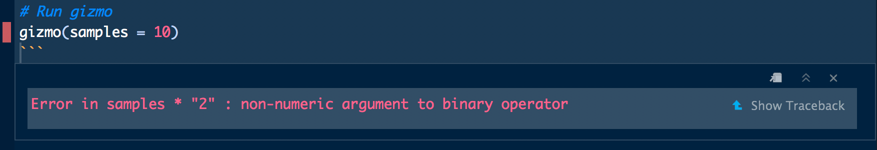
# Run gizmo
gizmo(samples = 10)## Error in samples * "2": non-numeric argument to binary operatorWe receive a familiar error message but no information about where in the gizmo() function the error is located other than that it contains the code snippet samples * "2". We could open gremlins.R and search for the code snippet samples * "2", but that could be pretty inefficient if gremlins.R is a large script. Enter traceback(), which will print the call stack location of the last uncaught error:
traceback()
# 2: rnorm(n = samples * "2") at gremlins.R#12
# 1: gizmo(10)
Running traceback() tells us the the error occurs at gremlins.R#12, or line 12 in gremlins.R. If you’re working in a RMarkdown document or notebook, the error message generated by the faulty code chunk provides a shortcut for running traceback().
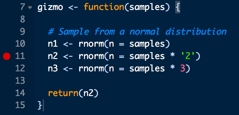
We can now open gremlins.R, navigate to line 12, and figure out what’s causing the error (which hopefully should be obvious at this point!).
Stop the code with breakpoints and browser()
In our previous example, the gizmo() function is very short and contains only one argument, samples = 10. Still, we can’t simply open gremlins.R and try to edit gizmo() because the samples variable only exists in gizmo()’s execution environment. Resist the temptation to create samples in your global environment! Doing so will likely lead to chaos down the line, especially when dealing with more complicated and/or nested functions. Instead, RStudio provides several handy tools for entering the current environment at any point in your workflow!
Breakpoints
The easiest way to stop on a given line of code is to create an editor breakpoint by clicking to the left of the number in the code editor. The breakpoint will be indicated by a solid red dot (or hollow dot to indicate the function has not yet been created) to the left of the line number
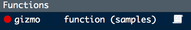
RStudio will also put a red dot next to the function name in the environment pane to indicate which of your functions currently have breakpoints
An advantage to using breakpoints is that they do not require saving or re-sourcing the function to take effect.
Browser
Another way to stop code on a specific line of code is with the browser() function. Unlike breakpoints, you must explicitly add the browser() statement to your code and update the function or script by calling source(). When the function is called, code execution will halt at the browser() statement.
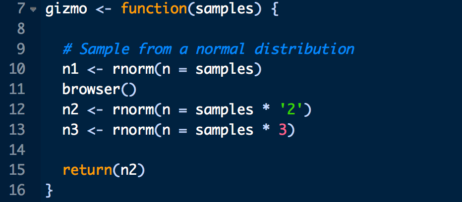
The advantage of using browser() over a breakpoint is, because browser() is part of the code, you can create conditional breakpoints. A good example of this is when an error occurs in the middle of a for() loop.
for(i in 1:10){
  # run function for working iterations
  do_something()
  # Add conditional browser to examine iteration generating error
  if(i == 6) {
    browser()
    do_something()
    }
}
Examine the code in debug mode
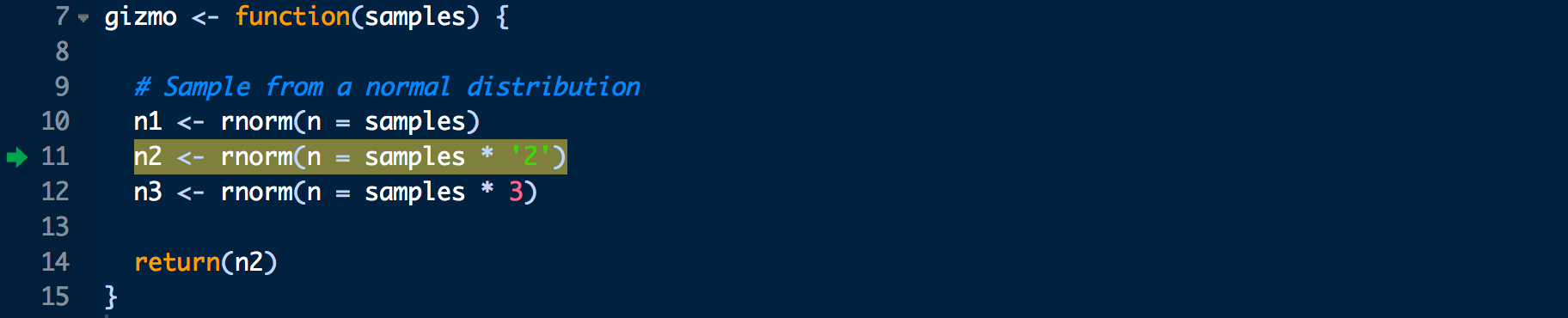
Once code execution is halted by a breakpoint or browser(), RStudio will enter debug mode and open the currently executing function.
At the same time, your console will now include a new toolbar for executing code and display Browse[1]> instead of the usual > to indicate you are in debug mode.
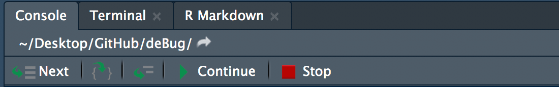
You’re now ready to troubleshoot the error in your code from within the execution environment. Good luck!